Studying makes you richer? (Advanced)

Does a longer education mean a higher salary?

What happens to the salary when you go from 12 years to 14 years? and from 14 years to 16 years?

Which one of these two is true: does your salary depend on your studies (or qualification), or does your salary determine how many years you studied?

How do you know, intuitively, if the line matches the data well or not? Are there any values you can calculate that tell you similar things?

Is there a linear correlation between the data? How strong is it? How do you know?

Are all the data points part of the trend line? How far are they? What does it tell you about the line?

Can a regression line predict unknown values?

Think about what it means in real life to study 24 years or 6 years. What jobs can you get with such education?

Can a yearly salary have any arbitrary value? Does it have an upper or lower limit?

How many data points do we have for less than 11 years studied? How many for more than 22?

Look at the answers to Question 3, do you see anything interesting?

Can an employer pay any salary to a worker? We are only paying attention to legal contracts.

How many years of studies would I need to expect a salary of 300 000 USD? Is that realistic?

They seem positively correlated: as one increases, the other increases (more or less) proportionally. The years studied is the independent variable since higher education opens opportunities in higher-paying jobs.

y = mx + b => y = 5786.51x - 35925.35 => yearly_income = 5786.51*years_studied - 35925.35
There are many ways to assess the fit of a linear regression line. Two of the most common methods are the correlation factor and the determination coefficient (R-Squared or R²).
For the correlation factor => we have r = 0.9983, which means a strong correlation between the variables.
For R-squared => we have R² = 0.9864, which means that the regression line describes the data very accurately.
Other possible parameters of analysis are the residues.

After 24 years of studies your expected salary is: 102,951 USD/year
After 6 years of studies, your predicted salary is: -1206.29 USD/year
While for 24 years of study the prediction seems reasonable, for 6 years of studies it is clearly wrong. Salaries cannot be negative and there are laws that put a lower limit on salaries.

We can only guarantee a certain level of accuracy within the range of our data, in our case 12-21 years. In this particular case, the upper range might follow the same linear trend, but only up to a point. There is a limit to how many years a person can study. Also, factors such as job experience become more important than education for very high-paying jobs.
On the lower end, salaries cannot be negative. Jobs that require no formal education still have to comply with the minimum wage regulations. For this reason, the linear relationship won’t describe the real situation accurately.

Since we want to infer if there is a correlation between our two variables without any calculations, we plot the points in a graph. We do it by hand or using one of the multiple tools available online (search for “Scatter plot”). The result will be something similar to the image next to the text. We can see that the points seem to align in a (roughly) straight line, which means there is a linear correlation between them.

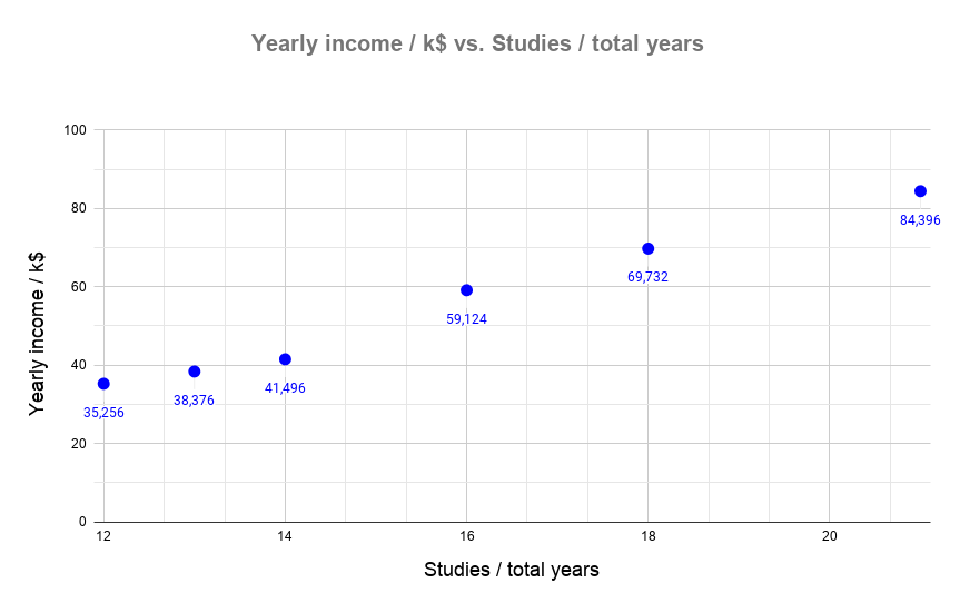
The correlation will be apparent no matter what we choose as the dependent/independent variable. However, we can safely assume that the money we earn can not change the number of years we have studied. The number of years you have studied can actually affect the amount of money you make since higher-paying jobs usually require a higher level of education (which means more years studying). That is why we have selected the years studied as the independent variable (x-axis) and the income as the dependent one (y-axis)

There are many techniques to calculate the regression line (or trend line) of a collection of points. The most commonly used is the least-squares method. This method minimizes the sum of the square of the distance from each point to the line. 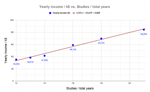Using the Least Squares Regression Line Calculator, we obtain the values for the slope as well as the y-intercept with their respective errors. These values are all we need to get the equation of a line in the slope-intercept form.
The result is that for a slope: m = 5790 while the intercept is b = -36000.
The equation of the line is:
y = mx + b => y = 5786.51x – 35925.35
using our variables we obtain:
yearly_income = 5786.51*years_studied – 35925.35

We can assess the goodness of a regression line by using many different parameters. We will focus on the correlation factor and the coefficient of determination (R²).
To obtain the numerical answer we want, we can simply use the Coefficient of Determination Calculator (R-squared) and the Pearson Correlation calculator.  The results are:
Correlation factor: 0.9983
R-squared: 0.9864
The correlation factor tells us the correlation between our variables, that is, how changing one variable affects the other. The correlation factor always has a value between -1 and +1 (both inclusive) with a higher absolute value indicating a stronger correlation. In our case, 0.9983 is a very strong correlation, almost perfect.
On the other hand, R-squared takes a value between 0 and +1, with the higher values indicating that the regression line is a very accurate description of the underlying relationship between our data points. A value of 0.9864 indicates that our points are almost part of the line. A typical interpretation of such a high value is that the trend line fits the data very well.

Now, we want to obtain the expected income for someone who has studied for 24 years. Since the trend line is what helps us predict values for missing data, we simply plug the number into the equation for the line:
yearly_income = 5786.51*years_studied – 35925.35 => yearly_income = 5786.51*24 – 35925.35 => yearly_income = 102951 USD
We can do the same for 6 years:
yearly_income = 5786.51*years_studied – 35925.35 => yearly_income = 5786.51*6 – 35925.35 => yearly_income = -1206.29 USD
While the value for studying 24 years seems reasonable, the expected salary after 6 years of studies is clearly incorrect. Not only because salaries are always positive (or zero for unemployed) but they also have to comply with minimum wage regulations, putting a lower limit on the yearly earnings.
This is our first peek at the importance of analyzing the results we get from the trendline and seeing if they make sense. Knowing the range in which we can make accurate predictions is as important as the predictions themselves.

We have seen from Question 3 that not all of our predictions are correct. To estimate the range of validity we first look at our data range. Within 12 to 21 years of education, we can be confident that our predictions will match with reality fairly accurately (see Question 2 for how accurately). Beyond those limits, we have to play a guessing game. 
Here are some examples or possible argumentations:

• At the lower levels, not having a high school degree is generally the cutoff point. We can assume that the jobs available for someone with no high school diploma are the same irrespective of when they dropped. 
• The validity of our predictions can be expected to hold for values slightly above 21 years. However, as we move higher and higher over that value the accuracy of our predictions will suffer. Job experience will become a very important factor, there is an upper limit to how many years a person can study, at some point salaries depend more on the responsibilities and power inherent to the position that to the qualification required.
• Minimum wage regulations and job availability can have an impact on the correlation above and below our data range.

More arguments can be made, so just think about it and come up with your own.